Bias and Fairness

7. Bias and Fairness#

Now that we have seen concrete examples of models and learning algorithms in both the settings of regression and classification, let’s turn back to the discussion we introduced at the beginning of the book about the use of ML systems in the real world. In the Introduction, we discussed a few examples of deployed ML models that can be biased in terms of the errors or the predictions they make. We highlighted the Gender Shades study that showed that facial recognition systems were more accurate on faces of lighter-skinned males than darker-skinned females. We also discussed the PredPol model that predicted crime happening way more frequently in poorer communities of color, simply by the choices of which crimes to feed the model in the first place and the feedback loops that creates.

You will have no trouble trying to find other examples of machine learning systems’ biased outputs causing harm. From Google’s ad algorithm showing more prestigious jobs to men, to Amazon’s recruiting tool that was biased against women, to the COMPAS model used in the criminal justice system falsely predicting Black individuals were more likely to commit crimes.

Clearly it is possible to spot model’s that behaviors are not ideal and the results in these headlines are clear signs of bias somewhere in our ML system. But the question is where does that bias come from? How does it effect our models? And importantly, what steps can we take to detect and hopefully prevent these biased outcomes from happening in the first place? In this chapter, we will highlight some of the current research into the workings of ML models when the interact with society, and how we can more formally define concepts of bias and fairness to prevent our models from causing harm before we deploy them.

This chapter will tell this story about defining bias and fairness in three major parts:

Background: The COMPAS Model
Where does Bias come from?
How to define fairness?

Before beginning this journey, it is important to note that my experience has being squarely from the field of machine learning and computer science. While many of these discussions of how to encode concepts of fairness into models are relatively new in our field (~15 years), these are not necessarily new concepts. Scholars of law, social justice, philosophy and more have all discussed these topics in depth long before we have, and we will only be successful by working with them in unison to decide how to build our models.

7.1. Background: The COMPAS Model#

A few years ago, a company called NorthPointe created a machine learning model named COMPAS to predict the likelihood that an arrested person would recidivate. Recidivation is when a person is let out of jail, where they eventually recommit that crime. Recidivating is an undesirable property of the criminal justice system, as it potentially means that criminals were being let go just to go repeat the crimes they were originally arrested for. So the modelers were hoping use data to better predict who was more likely to recidivate could help the criminal justice system. This model was deployed and was used by judges to help them determine details of sentencing and parole, based on how likely the person was predicted to be a risk of reoffending.

The modeling task COMPAS set out to solve was to take information about a person who was arrested, and predict how likely they would be to recidivate. The person who was arrested was given a survey asking questions about their life such as “Was one of your parents ever sent to jail or prison?” and “How many of your friends/acquaintances are taking drugs illegally?” Important to note for what will come up, the survey never asks the person about their race or ethnicity. The COMPAS model then takes this survey and computes a score from 0 to 10. This regression task indicates that a score near 0 is unlikely to recidivate and a score of 10 means they are very likely to recidivate. The training data for this model was based on survey results of past persons who were arrested and the labels to calibrate the scores were if that person was re-arrested in 2 years of being released.

ProPublica, an independent non-profit newsroom, did an analysis in 2016 that claimed that this COMPAS model was biased against Black people who were arrested. ProPublica’s piece outlines that the risk scores that COMPAS predicted for Black people were more likely to be in the “high risk” category (scores closer to 10) than White people with comparable backgrounds. That, along with other details, led them to the conclusion that this COMPAS model was biased against Black people.

Northpointe, the model’s creators, countered in their own article that the ProPublica analysis was flawed and that if you look at the data, the scores they predicted are well calibrated. Calibration is a measure for risk-score models like COMPAS to measure how likely their scores relate to the true probability of recidivating. So for example, a model is well calibrated if, when it predicts a risk score of 2/10, there is about a 20% chance that the person actually recidivates, as compared to when it predicts a score of 9/10, there is about a 90% chance that the person actually recidivates. So their claim is the that the model is in fact well calibrated, and their scores are accurate to reality¹.

So this leaves us with some key questions: Who is right here? Do either of these claims make us feel more or less confident about using a model like this in the criminal justice system?

Well, in a sense, they are actually both correct. At least, you can use the same data to back up both of their claims.

Consider Northpointe’s claim of the model being well calibrated. The following graph from the outputs of the model and comparing it to the rate of recidivism. The graph shows the calibration curve for the model separating its scores for Black/White people. Northpointe’s claim is that these scores are close to the line \(y = x\), meaning good calibration. And to bolster their point, the calibration is more-or-less the same across the groups Black/White. Clearly the lines aren’t exactly the same, but the gray error regions show uncertainty due to the noise in the data, and those regions of uncertainty overlap by a lot indicating the two trends are reasonably close given the amount of certainty we have.

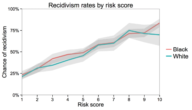
Fig. 7.1 Recidivism rate by risk score and race. White and black defendants with the same risk score are roughly equally likely to reoffend. The gray bands show 95 percent confidence intervals. (Source: The Washington Post)#

But it turns out that the same data can also back up ProPublica’s point! In particular, if you look at the rate of mistakes made by the model, it is more likely to label Black people who would ultimately not reoffend with a higher risk. Consider changing this problem from a regression one to a classification one, where the labels are “Low Risk” (negative) and “High Risk” (positive). In this setting, ProPublica is arguing that the false positive rate for Black people is much higher than the FPR for White people. This can be seen in the graph below, where a larger percentage of Black People who did not reoffend are disproportionately rated as higher risk.

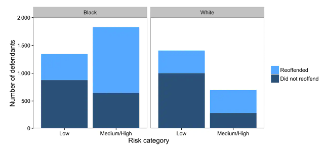
Fig. 7.2 Distribution of defendants across risk categories by race. Black defendants reoffended at a higher rate than whites, and accordingly, a higher proportion of black defendants are deemed medium or high risk. As a result, blacks who do not reoffend are also more likely to be classified higher risk than whites who do not reoffend. (Source: The Washington Post)#

In this graph, we can actually still see the truth of Northpointe’s claim. Within each category (low/high), the proportion that reoffended are the same regardless of race. But the fact that a larger shade of “Did not reoffend” (dark blue) are labeled High Risk for Black people is Propublica’s claim of bias.

So how can both actually be right? Well, as we will see later in this chapter, defining notions of fairness can be a bit tricky and subtle. As a bit of a spoiler for the discussion we will have over this chapter, there will never be one, right, algorithmic answer for defining fairness. Different definitions fairness satisfy different social norms that we may wish to uphold. It’s a question of which norms (e.g., non-discrimination) we want to enshrine in our algorithms that is the important discussion to be had, and that requires people with stakes in these systems to help decide. Our book, can’t possibly answer what those decisions should be in every situation, so instead, we are going to try to introduce the ideas of some possible definitions of bias and fairness and talk about how they can be applied in different situations. This way, you have a set of “fairness tools” under your toolbelt to apply to the situation based on what you and your stakeholders decide are important to uphold in your system.

7.2. Bias#

Before defining concepts of “what is fair”, let’s first turn to a discussion of where this bias might sneak in to our learning systems. Importantly, if we believe this COMPAS model is making biased outcomes, we should ask “Where does this bias come from?”

As we addressed in the Introduction, most times bias enters our model through the data we train it on (Garbage in \(\rightarrow\) Garbage out. Bias in \(\rightarrow\) Bias out). It probably wasn’t the case that some rogue developer at Northpointe intentionally tried to make a racist model. Instead, it is more likely that they unintentionally encoded bias from the data the collected and fed to the model. However, if you remember carefully, we said earlier on in the description of the COMPAS model that it doesn’t even use race/ethnicity as a feature! How could it learn to discriminate based on race if it doesn’t have access to that data?

The simple answer is even though it didn’t ask about race explicitly, many things it asks can be highly correlated to race. For example, due to historic laws that prevent Black families from purchasing property in certain areas in the past, continue trends today of certain demographics being overrepresented in some areas and underrepresented in areas. Zip code is a somewhat informative proxy of race. Now consider that with all of the other somewhat informative correlations you can find with race (health indicators, economic status, name, etc.) the model can inadvertently pick up the signal that is race from all of those proxy features.

The story of where bias enters our model is as bit more complex than just that though. It is worth diving in to the various points of our ML pipeline that can be entry points for bias to our model. Most of this section of the chapter is based on the incredible A Framework for Understanding Unintended Consequences of Machine Learning (Suresh & Guttag, 2020). In their paper, they outline six primary sources of bias in a machine learning pipeline that we will introduce and summarize. These sources are:

Historical bias
Represenation bias
Measurement bias
Aggregation bias
Evaluation bias
Deployment bias

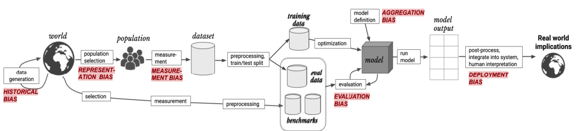
An ML pipeline with the sources of the six biases listed above — Fig. 7.3 An ML pipeline with the 6 sources of bias entering at various points.#

7.2.1. Historical Bias#

Historical bias is the reflection that data has on the real world it is drawn from. The world we live in is filled with biases for and against certain demographics. Some of these biases were ones that started a long time ago (e.g., slavery) that can have lasting impacts today, others are biases that emerge over time but can still be present and harmful (e.g., trans-panic). Even if the data is “accurately” drawn from the real world, that accuracy can reflect the historical and present injustices of the real world.

Some examples:

Earlier we introduced the concept of redlining. A common practice historical, illegal today, still has lasting effects due to housing affordability and transfer of generational wealth.
The violence against Black communities on the part of police make data in the criminal justice system related to race extremely biased against Black people.
In 2018 only about 5% of Fortune 500 CEOs were women. When you search for “CEO” in Google Images, is it appropriate for Google to only show 1 in 20 pictures of women? Could reflecting the accurate depiction of the world perpetuate more harm?

Historical bias is one of the easiest forms of bias to understand because it draws from the concepts of bias we understand as human beings. That doesn’t mean it is always easy to recognize though. A huge source of biases come from unconscious biases that are not necessarily easy for us to spot when they are in our own blind-spots.

7.2.2. Representation Bias#

Representation bias happens when the data we collect is not equally representative of all groups that should be represented in the true distribution. Recall that in our standard learning setup, we need our training to be a representative sample of some underlying true distribution that our model will be used in. If the training data is not representative, then our learning is mostly useless.

Some examples of representation bias in machine learning include:

Consider using smartphone GPS data to make predictions about some phenomena (e.g., how many people live in a city). In this case, our collected dataset now only contains people who own smartphones with GPSs. This would then underestimate counts for communities that are less likely to have smartphones such as older and poorer populations.
ImageNet is a very popular benchmark dataset used in computer vision applications with 1.2 million images. While this dataset is large, it is not necessarily representative of all settings in which computer vision systems will be deployed. For example, about 45% of all images in this dataset were taken in the US. A majority of the remaining photos were taken in the rest of North America and Western Europe. Only about 1% and 2.1% of the images come from China and India respectively. Do you think a model trained on this data would be accurate on images taken from China or India (or anywhere else in the world) if it has barely seen any pictures from there?

7.2.3. Measurement Bias#

Measurement bias comes from the data we gather often only being a (noisy) proxy of the things we actually care about. This one can be subtle, but is extremely important due to how pervasiive it is. We provide many examples for this one to highlight its common themes.

For assessing if we should give someone a loan, what we care about is whether or not they will repay that loan through some notion of financial responsibility. However, that is some abstract quantity we can’t measure, so we use someone’s Credit Score as a hopefully useful metric to measure something about financial responsibility.
In general we can’t predict the rate that certain crimes happen. We don’t have an all-mighty observer who can tell us every time a certain crime happens. Instead, we have to use arrest data as a proxy for that crime. But note, that arrest rate is just a proxy for crime rate. There are many instances of that crime that may not lead to arrests, and people might be arrested for not that crime at all!
For college admissions, we might care about some notion of intelligence for admissions to college. But intelligence, like financial responsibility, is some abstract quality not a number. We can try to come up with tests to measure something about intelligence, such as IQ tests or SAT scores and use those instead. But note those a proxies of what we want, not the real thing. And worse, those tests have been shown to not be equally accurate for all subgroups of our population; IQ tests are notoriously biased towards wealthier, whiter populations. It’s likely that these measure have nothing to do with the abstract quality we care about.
If factory workers are predicted that they need to be monitored more often, more errors will be spotted. This can result in feedback loops to encourage more monitoring in the future.
- This is the exact thing we saw with PredPol system in the introduction, where more petty crimes fed into the model led to more policing, led to more petty crimes being fed to the model.
Women are more likely to be misdiagnosed (or not diagnosed) for conditions where self-reported pain is a symptom since doctors frequently discount women’s self-reported pain levels. In this case “Diagnosed with X” is a biased proxy of “Has condition X.”

So measurement bias is bias that enters our models from what we choose to measure and how, and often that the things we measure are (noisy) proxies of what we care about or not even related at all!

In particular, we have actually tricked you with a form of measurement bias throughout this whole chapter to highlight how tricky it can be to spot. Recall when we introduced the COMPAS we said the goal was to predict whether or not someone would recidivate. Again, recidivating is recommitting the crime they were arrested for sometime in the future. How did Northpointe gather their training data for make their model? They looked at past arrests and found whether or not that person was arrested again within two years. Think carefully: Is what they are measuring the same as the thing they want to measure?

No. They are not the same. The data “arrest within two years” is a proxy for recidivating. Consider how they differ:

Someone can re-commit a crime but not be arrested.
Someone can be arrested within two years, but not for the same crime they were originally arrested for.
Someone can re-commit a crime more than two years after their original arrest.

Now consider all of the ways that those differences can affect different populations inconsistently. With our PredPol (predictive policing) example earlier, and the discussion of over-policing of Black communities. It is completely unsurprising that there is a higher arrest rate among Black people who previously were arrested, even if it wasn’t some recidivating (e.g., maybe they were originally arrested for robbery, but then re-arrested for something petty like loitering). This is one of the reasons why when you look at the COMPAS data, you see a higher “recidivism” rate for Black people. Because they aren’t actually measure recidivsim, they are measuring arrests!

Measurement bias sneaks in to ML systems in so many sneaky ways when model builders don’t think critically about what data they are including and why and what they are actually trying to model. A general rule of thumb is that anything interesting you would want to model about a person’s behavior rely on some, if not all, measures of proxy values.

7.2.4. Aggregation Bias#

Often times we try to find a “one size fits all” model that can be used universally. Aggregation bias occurs when using just one model fails to serve all groups being aggregated over equally.

Some examples of aggregation bias:

HbA1c levels are used to monitor and diagnose diabetes. It turns out HbA1c levels differ in complex ways across ethnicity and sex. One model to make predictions about HbA1c levels across all ethnicities and sexes may bne less accurate than using separate models, even if everyone was represented in the training data equally in the first place!
General natural language processing models tend to fail on accurate analysis of text that comes from sub-populations with a high amount of slang or hyper-specific meanings for more general words. As a lame, Boomer example, “dope” (at one point) could have been recognized by a general language model as meaning “a drug”, when younger generations usually say it to mean “cool” by a general language model as meaning “a drug”, when younger generations usually say it to mean “cool”.

7.2.5. Evaluation Bias#

Evaluation bias is similar to representation bias, but is more focused on how we evaluate and test our models and how we report those evalutions. If the evaluation dataset or the benchmark we are using doesn’t represent the world well, we can have an evaluation bias. A benchmark is a common dataset used to evaluate models from different researchers (such as ImageNet).

Some example of evaluation bias:

Similarly, the ImageNet example would also suffer from evaluation bias since its evaluation data is not representative of the real wrold.
It is common to just report a total accuracy or error on some benchmark dataset and using a high number as a sign of a good model without thinking critically about the errors it makes.
- We saw earlier in the Gender Shades example that there was drastically worse facial recognition performance when used on faces of darker-skinned females. The common benchmarks for these tests that everyone was comparing themselves on only had 5-7% faces of darker-skinned women.

7.2.6. Deployment Bias#

Deployment bias can happen when there is a difference between how a model was intended to be used, and how the model is actually used in real life.

Some example of deployment bias include:

Consider the context of predicting risk scores for recidivism rates. While it may be true that the model they developed was calibrated well (its scores were proportional to rate of recidivism), their model wasn’t designed or evaluated in the context of a judge using the scores to decide parole. Even if its calibrated in aggregate, how do they know how it performs on individual cases where a human then takes its output and then makes a decision. How the model was designed and evaluated didn’t match how it was used.
- People are complex, and often don’t understand the intricacies of modeling choices made by the modelers. They might make incorrect assumptions about what a model says and then make incorrect decisions.

7.2.7. Recap#

So now with a brief definition of all of these biases, it would be good to look back at this ML pipeline Suresh & Guttag introduced to get a full picture of how they enter and propagate throughout and ML system (Fig. 7.3).

7.3. Fairness#

Now that we have discussed sources of bias in our model, we have a clearer idea of precisely how they can enter our ML pipeline. While the outputs of the model being biased feels unfair, it turns out that we will not get fairness for free unless we can demand it from our models. What we are interested in exploring now is how to come up with mathematical definitions of fairness, such that we can compute some number(s) to tell us if biases in our model are ultimately affecting its predictions in an undesired way.

There is a lot of active research ³ on how to come up with mathematical definitions of fairness that we can enforce and verify. The hope is that by coming up with some mathematical definition, we can hopefully spot early in the process when the model might exhibit unfair outputs.

In this chapter, we will introduce a few different possible definitions of fairness, and afterwards we will look at comparing them to see if they can be cohesive. In particular in this chapter, we will be interested in coming up with definitions for a concept known as group fairness. Group fairness, also called non-discrimination is the intuitive concept that fairness means your membership of some group based on some uncontrollable property of yourself (race, gender, age, nationality, etc.) shouldn’t negatively impact the treatment you receive. Group fairness notions are ones that try to prevent discrimination such as racism, sexism, ageism, etc.

For the remained of this chapter, we are going to focus on a cartoonishly simplified example of college admissions to try to reveal the key intuitions of how we can potentially define fairness. Note that the assumptions in this example are clearly not correct, but we use it for its simplicity and to act as a proof of concept. The intent is that by showing behaviors and properties of an overly simplified, contrived scenario, we can better understand what we can expect in real life. All of the things we will introduce in this chapter an be generalized to the complexities of the real world.

Important

College Admissions - Credit This example is borrowed from the fantastic The Ethical Algorithm by Michael Kearns and Aaron Roth. This book is an incredible overview of the current work done to embed socially-aware values, such as fairness, into algorithms. We include their example scenario to introduce concepts of fairness because it is that good. Our contribution to the example is adding mathematical definitions and notation to make the ideas they present in this book for general audiences more suitable for a technical one.

So in this example, we are in charge of building a college admissions model. This model is supposed to take information about a college applicant, and predict whether or not we should let them in. In this scenario, we are going to make the following (unrealistic) assumptions:

The only thing we will use as an input to our model is the students’ SAT score. Clearly real college admissions systems use more information and include holistic reviews, but we will limit this for simplicity.
For every applicant, there is some single measurable notion of “success” and the goal of our model is to let in students who will meet this definition of success. Depending on the priorities of your college, you could imagine defining success as 1) will the student graduate, or 2) will the student graduate and get a job or 3) will the student graduate and give a ton of money back to the school. Depending on how you define success, that defines which examples are considered “positive” and “negative” examples. Clearly “success in college” is more complex than just one goal, as every individual student might have their own notion of what being successful in college means. For simplicity though, we will assume there is a consistent and universal notion of “successful college student”, whatever that may be.
There is no notion of competition or limited spots. If everyone would truly meet the definition success, then everyone would be let in. But that doesn’t mean we want to have our model let everyone in since if they ultimately wouldn’t be successful, that could be a huge waste of time and money for us and the student.
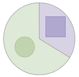
To talk about demographics and concepts of group fairness, we will assume all of our applicants are part of one of two races: Circles and Squares. In this world, Circles make up a majority of the population (66%) and Squares (33%). Consider that in this world Squares also face systematic oppression, and often are economically disadvantaged due to the barriers they face in their lives.

Now again, all of this is an extreme over simplification of the real world, but it will still be useful for us to get some key intuitions for what fairness might mean in the real world.

7.3.1. Notation#

Before defining fairness formally, we need to introduce some notation to describe the situation we defined above. In our ML system, our training data will be historical data of students and if they met our definition of success. Recall that the only input we will use in this example is the SAT score, but we will also track the demographics of Circle/Square to understand concepts of fairness. The notation will be general for more complex scenarios, and we highlight what values they take in our example

Notation

\(X\): Input data about a person to use for prediction

Our Example \(X = \text{SAT Score}\)

\(A\): Variable indicating which group \(X\) belongs to

Our Example: \(A = \square\) or \(A = \bigcirc\)

\(Y\): The true label

Our Example: \(Y = +1\) if truly successful in college, \(Y = -1\) if not

\(\hat{Y} = \hat{f}(X)\): Our prediction of \(Y\) using learned model \(\hat{f}\)

Our Example: \(\hat{Y} = +1\) if predicted successful in college, \(\hat{Y} = -1\) if not

7.3.2. Fairness Definitions#

In our setup, we might be concerned that our college admissions example may potentially be biased against Squares given the fact that they are a smaller portion of the population, and we may be concerned about the adverse affects of the discrimination they face in the world affecting our college admissions choices. But how can we definitively know what discrimination is or if our system is unfair? This is where we introduce the concept of coming up with measure to describe how fair a system is, and if we see that fairness is being violated, is a clear indicator that our system is discriminatory ⁴. We’ll see different

In the following sections, let’s explore some mathematical definitions of concepts of fairness using the notation we outlined above. Recall that we are focused on notions of group fairness, where we don’t want someone’s outcome to be negatively impact by membership in some protected group (in this case their race being Circle or Square).

We also show for each section a brief code example to show how to compute the numbers in question. The code examples assume you have a DataFrame data with the all of the data and predictions.

X	A	Y	Y_hat
…	…	…	…

7.3.2.2. Statistical Parity#

So since being completely unaware of race to achieve fairness wasn’t feasible, let’s explore notions that try to compare how the model behaves for each of the groups of our protected attribute \(A\). The simplest notion to compare the behavior on groups is known as statistical parity. Statistical parity dictates that in order for a model to be considered fair, the predictions of the model need to satisfy the following property.

\[P(\hat{Y} = +1 | A=\square) \approx P(\hat{Y} = +1 | A=\bigcirc)\]

In English, this says that the rate that Squares are admitted by our system should be approximately equal to the rate that the rate that Circles are admitted. So for example, if the admitted rate for Squares is 45%, then the admitted rate for Circles should be 45% as well. Note that we use approximately here and in other definitions because demanding exactly equal probabilities is often hard. Instead we usually define a range of acceptable distance such as 0.1% and won’t call it biased if the Square admission rate is 45% and the Circles is 45.1%.

Let’s consider some tradeoffs of using this definition to define if our admissions model is fair.

Pros

The definition is simple, and easy to explain. This is a positive because now users can better understand what we are measuring and when this definition of fairness is violated.
It only depends on the model’s predictions, so can be computed live as the model makes new predictions.
This definition aligns with certain legal definitions of equity so there is established precedent in it being used.

Cons

In some sense, it is a rather weak notion of fairness because it says nothing about how we accept these applicants or if they are actually successful. For example, a random classifier satisfies this definition of fairness even though it completely disregards notions of success. There are other, more nefarious, models that could be used that still meet statistical parity such as a classifier that is accurate for Square applicants, and then just chooses the same percentage of non-successful Circle applicant. It doesn’t seem fair that you can set up the Circles to fail even though they are equally represented.
- Do note that that the fact that a random classifier can satisfy this definition fairness is actually not all that much of a critique. In fact, it is a proof of concept that it is even possible to satisfy this definition of fairness. There are some useful notions of fairness which might not have algorithms that can actually satisfy them!
A more serious objection is that, in some settings, the rates for our labels might not be consistent across groups. Statistical parity is making the statement that the rates that which groups meet this positive label (collegiate success in our example), is consistent across groups. To be clear, it is very possible that the rates of success across groups is actually the same, but it’s possible that it’s not and forcing statistical parity in that case might not be right.

Let’s consider a different example to make that last point clearer. Consider a model that predicts if someone has breast cancer, and a positive label is the detection of breast cancer. Would we say the breast cancer model is discriminatory because \(P(\hat{Y} = +1 | A = \text{woman}) = 1/8\) while \(P(\hat{Y} = +1 | A = \text{man}) = 1/833\)? No, because clearly the base-rate of the phenomena we are predicting is different between men and woman. Forcing statistical parity in this model to consider it fair would mean either incorrectly telling more women they don’t have breast cancer (when they might actually) or telling more men that they do have breast cancer (when they in fact do not). In the case where the base rates differ, demanding statistical parity makes no sense.

Back our college admissions example, the same critique could apply if we assume the base rates of success are different. However, many people argue that in the college setting, the base rates for success should be equal enough (i.e., race does not effect your success in college), so statistical parity is appropriate. We will see later, how this assumption is a statement of a particular worldview about how fairness should operate.

The following code example shows how to compute the numbers we care about for statistical parity.

squares = data[data["A"] == "Square"]
circles = data[data["A"] == "Circle"]
square_admit_rate = (squares["Y_hat"] == +1).sum() / len(squares)
circle_admit_rate = (circles["Y_hat"] == +1).sum() / len(circles)

assert math.isclose(square_admit_rate, circle_admit_rate, abs_tol=0.01)

7.3.2.3. Equal Opportunity#

To account for the critiques of statistical parity ignoring the actual success of the applicants, we arrive at a stronger fairness definition called equal opportunity or the equality of false negative rates (FNR).

Equal opportunity is defined as the following. Recall that a false negative and true positive are the only possibilities when we are considering the true label are positive.

\[P(\hat{Y} = +1 | A=\square, Y=+1) \approx P(\hat{Y} = +1 | A=\bigcirc, Y=+1)\]

Note that this definition is almost the same as statistical parity, but adds the requirement that we only care about consistent treatment of Squares/Circles that were ultimately successful. In English, this is saying the rate that successful Squares and successful Circles are admitted should be approximately equal.

The intuition here is to remember our discussion on the relative costs of false negatives and false positives. If in our setting of college admissions, we assume the cost of a false negative (denying someone who would have ultimately been successful) is worse, then a reasonable definition of fairness would demand that the rate of those false negatives should be approximately equal across subgroups. Note that the definition above is about true positive rate (TPR) which is related to FNR by \(TPR + FNR = 1\).

As its own definition of fairness, equal opportunity has its own set of pros/cons in its use.

Pros

Much better since it controls from the true outcome. Fixes all of the cons of statistical parity.

Cons

This definition only controls for equality in terms of the positive outcomes. It doesn’t make any care about fairness in terms of the negative outcomes.
It is more complex to explain to non-experts. With even a little complexity, challenges can occur since its important everyone understands and agrees on what is at stake to be considered fair.
It requires actually knowing the true labels. This is fine to check if your model is unfair on the training data, but it is not possible to actually measure equal opportunity on new examples if you don’t know their true labels.

success_squares = data[(data["A"] == "Square") & (data["Y"] == +1)]
success_circles = data[(data["A"] == "Circle") & (data["Y"] == +1)]

# Note TPR + FNR = 1
tpr_squares = (success_squares["Y_hat"] == +1).sum() / len(success_squares)
tpr_circles = (success_circles["Y_hat"] == +1).sum() / len(success_circles)

assert math.isclose(tpr_squares, tpr_circles, abs_tol=0.01)

7.3.2.4. Predictive Equality#

Just like equal opportunity, predictive equality or the equality of false positive rate (FPR) takes the same form but for controlling the rate for negative examples. All of the commentary is the same for predictive equality but which numbers you compute are different. Useful when you care more about controlling equality in the negative outcome.

\[P(\hat{Y} = -1 | A=\square, Y=-1) \approx P(\hat{Y} = -1 | A=\bigcirc, Y=-1)\]

no_success_squares = data[(data["A"] == "Square") & (data["Y"] == -1)]
no_success_circles = data[(data["A"] == "Circle") & (data["Y"] == -1)]

# Note TNR + FPR = 1
tnr_squares = (no_success_squares["Y_hat"] == -1).sum() / len(no_success_squares)
tnr_circles = (no_success_circles["Y_hat"] == -1).sum() / len(no_success_circles)

assert math.isclose(tnr_squares, tnr_circles, abs_tol=0.01)

7.3.3. Which Metric Should I Use?#

Here we’ve just outlined 3, but there are many many more definitions you can consider.

So which one should you use? Or more specifically, considering our COMPAS example which one would we use to measure as a determination of the models predictions are fair or not?

Unfortunately, we cannot tell you in general. The reason is each definition makes its own statement on what fairness even means. Choosing a fairness metric is an explicit statement of values that we hold when thinking about fairness. Many of these values are important values, but are fundamentally assumptions about how we believe the world works. These assumptions are often unverifiable. Later in this chapter, we will explore contrasting worldviews and how they impact our understanding of fairness.

7.3.4. How do I Use These Metrics?#

That is a simpler question to answer. A simple approach is to use them as part of your model evaluation. When comparing models of different types and complexities, you can use the metric of your choice to report a measure of each model’s fairness on both the training set and some validation set. Depending on your context, you might demand a certain threshold for your fairness metric before deploying your model.

There are also techniques to augment our standard learning algorithms to make them fairness-aware in the first place. Some algorithms are more complex than others, but they simply involve changing how we measure quality to care about fairness instead of just minimizing error. One simple approach is to use regularization, but instead of penalizing large coefficients, penalize coefficients that lead to larger disparities in some fairness metric.

7.4. (Im)Possibility of Fairness#

So while we have stated there is no single definition of fairness to use, since it depends on your context and values, one idea is to just satisfy them all! That seems like a good idea to form some super notion of fairness out of all of the individual definitions you could come up with.

For example, what if we wanted to make our model meet the following four definitions of fairness:

Statistical parity
Equal opportunity (equality of false negative rates)
Predictive equality (equality of false positive rates)
(Not yet discussed) Equally high accuracies of the model across the subgroups

It turns out with even just four notions of fairness at once, you cannot satisfy them all simultaneously unless the distribution of the subgroups are exactly the same. Unfortunately, due to all of the sources of bias we introduced above, this rarely happens in practice. What this means is that in the real world where we are working with biased data, we have to choose which fairness definitions to use since we can’t satisfy them all. This is often cited as a fairness “impossibility theorem” (example).

7.4.1. Fairness and Accuracy#

Important

The following example and graphic for this section is borrowed from the The Ethical Algorithm by Michael Kearns and Aaron Roth.

We can see a special case of this impossibility as the general observation that we see a tradeoff between accuracy and fairness in our models. In general, constraining our models to be more fair will make them less accurate. Let’s see an example as to why this might happen.

Continuing with our over-simplistic college admissions example, let’s add the following details:

The majority of the population (2/3) are Circles and remaining population (1/3) are Squares.
SAT scores for Circles tend to be inflated when compared to SAT scores of Squares. One possibility for why this could happen is that systematic barriers prevent Squares from accessing SAT prep at the same rate as Circles.
Despite this statistical difference in SAT scores, the rate that they are actually successful in college are the same.

Consider a toy dataset below that encodes these three assumptions. Students are plotted on a number line based on their SAT scores and are indicated by 1) Circle/Square and 2) +/- for if they were ultimately successful. If you count out all of the examples, you can see all three conditions above are true.

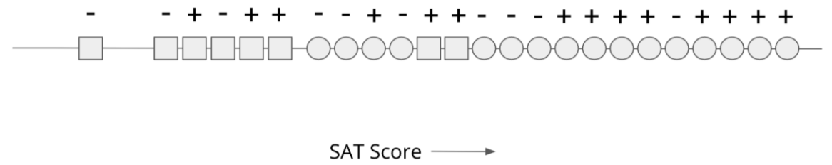
A numberline of circles and squares based on SAT score (described above). — Fig. 7.4 A toy example for our college admissions scenario (source: The Ethical Algorithm)#

Now if we phrase this as a machine learning problem, one of the simplest models is a simple threshold model that admits everyone above some chosen SAT score. We could find the “Optimal” threshold by trying out all of the thresholds and comparing them based on classification error. Note that in this case, there are finitely many thresholds to consider since with \(n\) data points, there are \(n + 1\) distinct thresholds that separate the points on the number line differently. The figure below shows the threshold that has the lowest classification error.

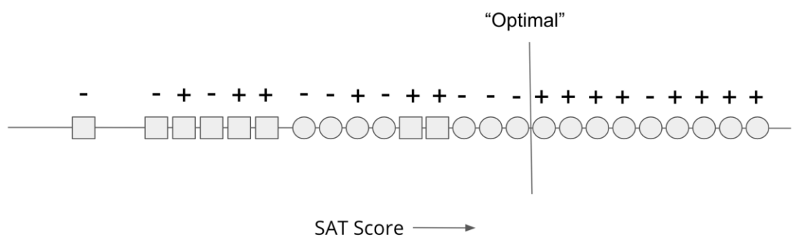
A numberline of circles and squares based on SAT score (described above) with a threshold labeled "Optimal". — Fig. 7.5 The optimal threshold for our toy scenario (source: The Ethical Algorithm)#

If you wanted to check the math, you would see that the accuracy of this threshold is \((8 + 9) / 24 \approx 70%\) since correctly let in 8 successful applicants and denied 9 unsuccessful ones. Any other threshold would make more errors and would be less accurate, so this one is considered “Optimal” for our training set.

But what if we wanted to consider how fair this model was? Let’s consider the definition of equal opportunity (or the equality of false negative rates).

\(P(\hat{Y} = -1 | A=\bigcirc, Y=+1) = \frac{1}{8 + 1} \approx 11%\)
\(P(\hat{Y} = -1 | A=\square, Y=+1) = \frac{0}{5 + 0} = 100%\)

So in terms of the false negative rates, this model seems completely unfair since it only falsely rejected 1/9 of the successful Circle applicants and all of the successful Square applicants. So this “optimal” model with the lowest classification error doesn’t satisfy equal opportunity.

Consider a lower threshold shown in the figure below labeled “More fair”.

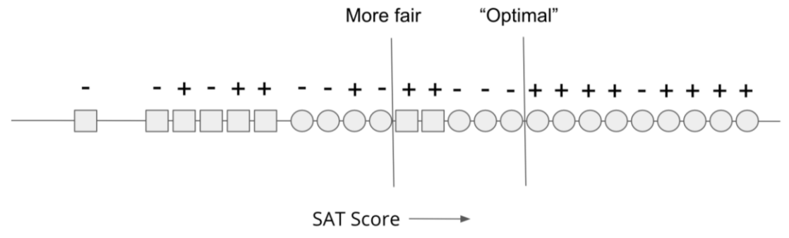
A numberline of circles and squares based on SAT score (described above) with a threshold labeled "Optimal" and a threshold labeled "More fair". — Fig. 7.6 The more fair threshold for our toy scenario (source: The Ethical Algorithm)#

We can run the same computation to see that this threshold is more fair according to equal opportunity.

\(P(\hat{Y} = -1 | A=\bigcirc, Y=+1) = \frac{1}{8 + 1} \approx 11%\) is unchanged since we didn’t let in any more successful Circles
\(P(\hat{Y} = -1 | A=\square, Y=+1) = \frac{3}{2 + 3} = 60%\) since we have now admitted 2 of the successful Squares

This model is more fair when defined by equal opportunity than the first model that we claimed was “optimal”. Note that this model is not necessarily fair since the FNR still are quite different, but it is more fair than the first model.

But what if we consider the accuracy of this “more fair” model? Well by making the model more fair, we have actually decreased the accuracy of the model since it let more unsuccessful Circles. The accuracy of this second model is \((9 + 5) / 24 \approx 66.7%\) which is lower than the first.

So in this toy example, we just saw that an increase in fairness was accommodated by an decrease in accuracy as well. You might argue that this is a result of our example being overly simplistic (and it is!), but this example is meant to by more of a proof-of-concept. The idea here is that this toy example shows the existence of a behavior even in a simple setting, implies it can happen in a real setting with more complexity. If you have doubts that this could happen in a real setting, consider all of the examples we pointed out at the beginning of this chapter of ML systems exhibiting biased outcomes. Those cases happened in the setting where we were trying to minimize classification error in the first place.

Our original quality metrics care about minimizing error, and as a result, we saw biased outcomes that it made. Controlling for fairness would result in a different model than the one we would have originally found, which is by definition, a model with more error than that biased model. Intuitively this happens because the data we train and evaluate ourselves on contains bias. Our definition of accuracy on that biased data, will require that being accurate means our model is biased.

In our toy example, the source of the problem was the artificial difference in SAT scores having no relation with the rate of success in college. In other words, the same scores are across Circles/Squares are not equally predictive of success. That difference is the source between this fairness and accuracy tradeoff. One way to address this problem is to recognize that statistical difference has no impact on the target we care about, and use different thresholds for each race. The figure below shows a two-threshold model and you can see that it has better fairness and accuracy in the predictions it makes.

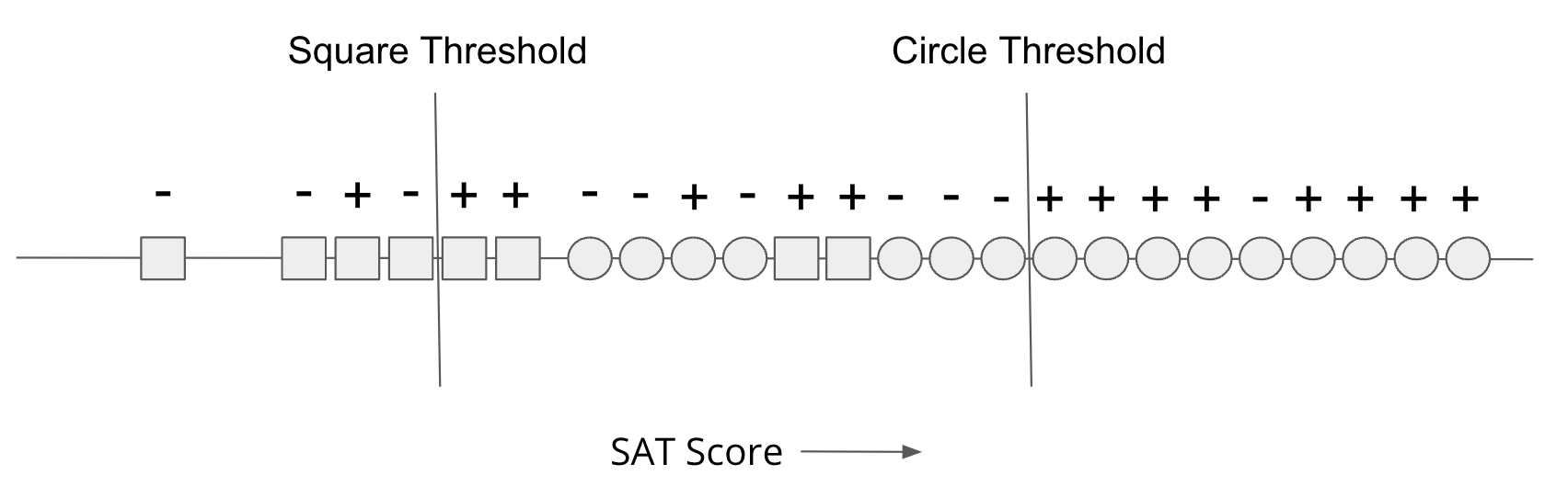
A numberline of circles and squares based on SAT score (described above) separate thresholds — Fig. 7.7 Using separate thresholds#

While this model that accounts for bias explicitly by using separate models for each group does avoid this fairness/accuracy tradeoff, it might not be the solution to the problem. There are two main difficulties using a model like this one.

(Legal) In many contexts, it is illegal to use race explicitly as an input to change outcomes. For example, it is illegal to use race as a factor in Credit Score computations. These laws are usually well intentioned to prevent discrimination by preventing racist decision makers from being able to use race as an input. But unfortunately, those same laws stop those trying to fight bias use more tailored models to prevent the biases in data from leaking into the model’s outcomes.
(Social) Despite this model being strictly better in terms of performance, it is often difficult to convince everyone that this model is actually better. In particular, many people argue that this model is in fact unfair because it lets admits “less qualified squares” an an affront to some concept of “merit”. This claim is exacerbated in the real world where colleges can’t admit everyone they predict will be successful and there is a notion of constrained seats. This causes a lot of debate over admissions policies that try to explicitly account biases present in the world. We’ll come back to this discussion near the end of the chapter to discuss the idea of worldviews and how to choose what is fair and unfair in them.

7.4.2. The Frontier of Fairness#

To visualize this tradeoff between fairness and accuracy more explicitly, we can consider every possible threshold and compare some metric for how much error it makes and how unfair it is. So for every possible threshold, we will compute the following two numbers:

\(error(w)\) = the classification error made by threshold \(w\)
\(unfair(w) = |FNR_{Square}(w) - FNR_{Circle}(w)|\) is the difference in the false negative rates. Intuitively a high difference in FNRs means the model is more unfair under equal opportunity.

So if we compute these numbers for every possible threshold, we can actually plot them out on a scatter plot where the x-axis is the error score and the y-axis is the unfairness score. Every possible model we considered would be one point on this graph that define its \((error, unfairness)\). The models in the top-right are models with high error and high unfairness, the models on the bottom right have high error and are more fair, and the models on the top left are more unfair but more accurate.

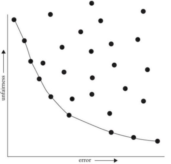
A depiction of the model performances (described above) and the Pareto frontier (described below). — Fig. 7.8 The fairness accuracy tradeoff and the Pareto Frontier (source: The Ethical Algorithm)#

Now while each model technically represents a different tradeoff between fairness and accuracy, it turns out that some of the models are definitively worse than others and should not be considered. For example, the top-right model that has high error and high unfairness would never be chosen since it doesn’t do well at either. Additionally, by moving from that model to another more to the down-and-to-the-left, you could improve its accuracy and fairness without hurting another. The same can’t be said for other models though, such as the one in the top left; you can improve that models unfairness, but that would come at a cost of increasing error (moving to the right).

The subset of these models that can’t be improved in one dimension without making the other dimension worse comprise an interested set of unique tradeoffs between fairness and accuracy. We call these models on the Pareto Frontier to represent how they are the “interesting” models to consider the require choosing between fairness and accuracy. In the figure above, they are draw on a curve towards the bottom-left of the figure. In some sense, a Pareto Frontier defines the only models we actually need to consider, because any other model could be improved to one on the frontier. Importantly, the Pareto frontier does not tell you which of the models on the frontier to use, it just shows you that there are many models that represent different tradeoffs in fairness and accuracy.

Michael Kearns and Aaron Roth provide the best commentary on Pareto Frontiers and how it might feel a bit weird to be so quantitative when considering if we care more about error or fairness. They write

While the idea of considering cold, quantitative trade-offs between accuracy and fairness might make you uncomfortable, the point is that there is simply no escaping the Pareto frontier. Machine learning engineers and policymakers alike can be ignorant of it or refuse to look at it. But once we pick a decision-making model (which might in fact be a human decision-maker), there are only two possibilities. Either that model is not on the Pareto frontier, in which case it’s a “bad” model (since it could be improved in at least one measure without harm in the other), or it is on the frontier, in which case it implicitly commits to a numerical weighting of the relative importance of error and unfairness. Thinking about fairness in less quantitative ways does nothing to change these realities—it only obscures them.

Making the trade-off between accuracy and fairness quantitative does not remove the importance of human judgment, policy, and ethics—it simply focuses them where they are most crucial and useful, which is in deciding exactly which model on the Pareto frontier is best (in addition to choosing the notion of fairness in the first place, and which group or groups merit protection under it, […]). Such decisions should be informed by many factors that cannot be made quantitative, including what the societal goal of protecting a particular group is and what is at stake. Most of us would agree that while both racial bias in the ads users are shown online and racial bias in lending decisions are undesirable, the potential harms to individuals in the latter far exceed those in the former. So in choosing a point on the Pareto frontier for a lending algorithm, we might prefer to err strongly on the side of fairness—for example, insisting that the false rejection rate across different racial groups be very nearly equal, even at the cost of reducing bank profits. We’ll make more mistakes this way—both false rejections of creditworthy applicants and loans granted to parties who will default—but those mistakes will not be disproportionately concentrated in any one racial group.

—The Ethical Algorithm, Michael Kearns and Aaron Roth

7.5. Fairness Worldviews#

In the concluding section of this chapter, we want to circle back on a discussion we have been putting off for most of the chapter involving thinking about the worldviews or assumptions we make when we are making certain fairness claims. So far we have focused on notions of group fairness or non-discrimination, but there are other forms of fairness we might consider. This last section is based primarily on the discussion in Friedler et al. (2016) that provides a framework for us to reflect on the assumptions we are making about our machine learning process and the data we train them on.

7.5.1. Moving Spaces#

The first thing they outline in this paper is a framework for more concretely thinking about how we model a learning task, and the assumptions we make along the way. Most learning tasks (including ones we have introduced in this book) start with the data we’ve gathered about the world, and then discuss modeling choices and algorithms to make predictions about the future.

In their paper, Friedler et al. argue there is actually a more nuanced story there, that brings to question what things we can even measure in the first place. They outline the learning process as a mapping between three spaces. As sub-bullets, we give a concrete example of these spaces in an example related to college admissions.

The Construct Space: True quantities of interest that we would like to measure, but we don’t actually have access to.
- College Admissions Example: What we actually care about in college admissions is measuring notions of intelligence, grit (perseverance), teamwork, leadership, etc. These are all qualitative and abstract concepts that don’t have a precise definition for measurement.
The Observed Space: The data we actually gather to use in our model are all proxy measurements to (hopefully) represent the constructs we care about. These proxies may or may not be good measures and they might also be noisy measurements of the constructs we care about. Importantly, we can’t verify if these proxies are good or not since we don’t have access to the Construct Space to verify the measurements are good ones.
- College Admissions Example: The data we actually gather for college admissions are your grades, your SAT/ACT scores, how many clubs you were a part of, other extra curriculars, etc. All of these hopefully give signal into the constructs we care about, but again, there is no way to actually verify that claim.
The Decision Space: We then use our learning model trained on the data in the Observed Space to make predictions in the Decision Space, or the set of possible outcomes we are predicting.
- College Admissions Example: The learning algorithm could be any classification algorithm and the Decision Space is decision Admit/Deny.

This process is depicted in the following graphic.

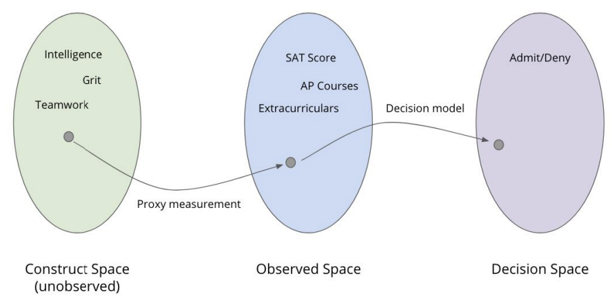
The Construct Space, Observed Space, and Decision Space (described above) — Fig. 7.9 The Construct Space, with Proxy Measures leading to the Observed Space, and the Decision Model leading to the Decision Space.#

7.5.2. Individual Fairness#

With this setup, we can now come up with a definition of fairness that also seems intuitive for us to try to follow named individual fairness. The intuition for this is that two people who look similar in the Construct Space should receive similar decisions in the Decision Space. Let’s try to define this formally.

Suppose we have a model \(f: CS \gets DS\) that maps values from the Construct Space (CS) to the Decision Space (DS). \(f\) is said to be individually fair if objects close in CS (based on some distance metric \(d_{CS}\)) end up close in DS (based on some distance metric \(d_{DS}\)). Specifically, \(f\) is \((\varepsilon, \varepsilon')\)-fair if for any \(x, y \in CS\)

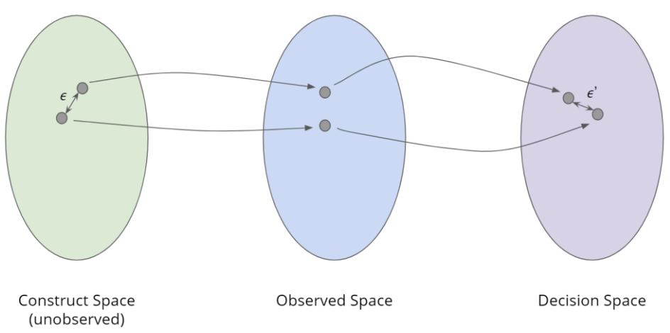
\[d_{CS}(x, y) \leq \varepsilon \rightarrow d_{DS}(f(x), f(y)) \leq \varepsilon'\]

A pictorial representation of individual fairness showing points close in the construct space being close in the decision space. — Fig. 7.10 Individual fairness#

Recall though, that we don’t have access to the Construct Space (CS). That means there is no way to verify individually fairness unless you make an assumption about how you believe the world works. When we care about individual fairness, we have to make an assumption known as What You See is What You Get (WYSIWYG). WYSIWYG is the assumption that the Observed Space (OS) is in fact a good measurement of the Construct Space. So for example, that means we are making the assumption that some numeric measurement such as SAT score is a good indicator for something like intelligence that we care about in the Construct Space (CS).

Under this assumption, we modify the definition above to measure the inputs in the Observed Space (OS) and now we have verifiable algorithm. Again, it’s only okay to do this because we are assuming the Observed Space is a good stand-in for the Construct Space. Under the WYSIWYG, you can easily compute the distances in Observed and Decision Spaces and report any unfairness when two applicants who are sufficiently close in the observed space get different decisions. In the College Admissions example, that case is when two students with similar SATs, grades, extracurricular activities, etc. get different admission decisions.

Aside: Discrete Decisions

One of the first results in Friedler et al. (2016) is to show that arbitrary individual fairness is not possible in the case that the decisions are discrete or categorical. The reasoning being if our construct space are real numbered values but our decision space is categorical, we can make two people arbitrarily close in the construct space that end up on opposite ends of the decision boundary.

This is a common complaint by students when course grades are assigned. In some instances, one student who had a 94.6% got an A and a student who had a 94.5% got an A-. The dividing line has to be somewhere and when there are a lot of students, the distance between two students on opposite ends of the line can be quite small. But if the decision space were real numbers, this is not an issue since you could make them just as close in the decision space as well.

7.5.3. Structural Bias#

But what if can’t assume that the Observed Space is a good measurement of the Construct Space? What if we instead assume that there is some presence of structural bias that might make people that are close in the Construct Space (CS) look very different in the Observed Space (OS). What if that structural bias impacts certain groups dispraportionately than others?

For example, SAT doesn’t just measure intelligence but also your ability to afford SAT prep. People who are just as intelligent (similar in Construct Space), might end up looking worse in the Observed Space because they don’t have the means to prepare and improve their SAT scores. So that means if a group is more likely to be economically disadvantaged due to current or historical barriers, then we would expect a distributional shift in their SAT scores looking worse despite them being just as intelligent.

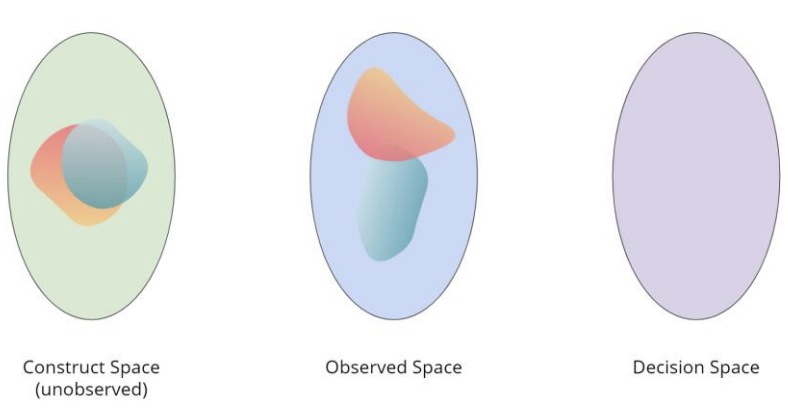
Showing a shift in distribution from the Construct Space to Observed Space — Fig. 7.11 Groups that are similar in the Construct Space may look different in the Observed Space due to structural bias#

When assuming the presence of structural bias, we normally also assume another claim that We’re All Equal (WAE). The WAE assumption states that all groups (e.g., race or sex) are equal enough that membership in that group should not make a meaningful difference for the task at hand (e.g., collegiate success). This is not saying the groups have to be exactly equal in every single way, but those differences are small and/or not related to the task at hand. In the college admissions example, the WAE attributes differences we see in SAT scores across races as the cause of structural bias instead of, say, that one race is “more intelligent” than another.

When assuming structural bias and WAE, we commonly think of fairness in terms of the group fairness definitions we defined before. Since we assume structural bias might make one group look better/worse in a way unrelated to the task at hand, then making sure membership in that group doesn’t disproportionally affect the decisions.

7.5.4. Which Worldview?#

So which worldview is right? WYSIWYG or structural bias + WAE? Unfortunately that question doesn’t really make sense or have an answer. They are worldviews. They are assumptions or beliefs about how you think the world works. How you think the world operates dictates if you think WYSIWYG or WAE in the face of structural bias. More importantly, which worldview you take determines what fairness means and which actions you deem unfair.

If you assume WYSIWYG, then individual fairness is easy to achieve. Recall WYSIWYG says the Observed Space is a good measure of the Construct Space. But under this world view, that means any attempt at group fairness or non-discrimination seem unfair because they may violate individual fairness (people that have similar data should get similar results). This worldview and critique of group fairness is the argument against policies such as affirmative action that people make: “My high achieving child didn’t get in because someone ‘less qualified’ did”. This statement is rooted in the assumption that the measurements of “high achieving” and “less qualified” are actually meaningful measurements, instead of having structural bias interfering.

On the other hand, if you assume structural bias + WAE, then group fairness is the right thing to do and we have seen many such group fairness mechanisms to ensure it. However, in this worldview attempts to achieve individual fairness may potentially cause discrimination. But in a lot of cases, it’s incredibly difficult to argue against this worldview with the sheer amount of evidence of structural barriers that our society puts up for certain groups.

7.6. Takeaways#

So what can we do with what we have learned in this chapter? Unfortunately we don’t have a concrete set of action items or algorithms here and we are more asking for a call to action to think critically about the impacts and assumptions of your model.

We clearly saw the importance of considering the impacts ML systems can have on society, both the positive and the negative. If we are not careful, these models can perpetuate, and worse, amplify injustices in our society.

A lof of work in the past decade or so has gone into defining concepts of bias and fairness more formally so that we can make our models less dangerous. While there is a lot of progress and exciting ideas in this space, the most important lesson that keeps resurfacing is there is not going to be a universal definition of fairness or algorithm to fix the problem. Instead, this is a crucial problem that we will need to rely on humans (not just ML engineers) in the loop to determine which properties of the system we will want. These are a question of human values, and we need informed humans to make those decisions.