8. Naïve Bayes#
While we have learned a lot about machine learning and ML models so far, our scope has been fairly narrow considering models that follow a similar structure. For both classification and regression, we have mostly talked about linear models that take the form of some coefficients \(w\) that we multiply with feature values to make some prediction \(w^Th(x)\). While there were some adjustments we had to make to that model in the classification setting to get Logistic Regression, the models we have discussed have had remarkable similarities.
While linear models are very popular and commonly used, they are not the only type of model. Now that we have a lot of the ML fundamentals down, we can now start introducing you to the wide world of various ML models. Each chapter from now on, more or less, will introduce a completely new type of model that makes different assumptions about how the world works. In this chapter, we will introduce the Naïve Bayes model for classification.
Learning Tip
With new models being introduced all of the time, it’s important to form a mental map of the concepts you are learning. Whenever we introduce a new model, make sure you reflect on how it relates to previous models or concepts we have discussed before. How are they similar? How are they different? What scenarios should one concept be used over another?
8.1. Probability Predictions#
At extremely high level, Naïve Bayes is similar to Logistic Regression in that it tries to predict probabilities of the form:
Where they differ, however, is in the details of how this probability is actually computed. Recall that Logistic Regression learned a linear Score model and converted Scores to probabilities with the sigmoid
Naïve Bayes will take a very different approach to computing these probabilities though. Instead of learning a linear model, it uses a theorem from probability about conditional probabilities called Bayes Theorem.
8.1.1. Bayes Theorem#
Bayes Theorem is an extremely well-known result in probability theory concerning conditional probabilities \(P(A|B)\). In English, this statement reads “The probability of A happening, conditioned on the fact that you know B happened.” So for example \(P(Raining|Umbrella)\) means the probability it is raining outside given the event that I have an umbrella with me.
How do we think \(P(A|B)\) relates to \(P(B|A)\)? Should they be the same? Or would they be different? Consider the rain and umbrella scenario. Is the likelihood of the two events the same?
The likelihood that it is raining (A), given the fact that I have an umbrella on me (B)
The likelihood that I have an umbrella on me (B), given the fact that it is raining (A)
Clearly these probabilities are related since I usually don’t carry an umbrella out when it is sunny, but we wouldn’t expect these probabilities to be exactly the same. In fact, Bayes Theorem gives a mathematical formula for how to convert between these two statements since they differ in value.
This formulation is incredibly useful because often times it is difficult to calculate \(P(A|B)\), but might be easier to compute the other values such as \(P(B|A)\), \(P(A)\), \(P(B)\).
8.2. Naïve Bayes#
Back to our discussion of our probability classifier, and how Naïve Bayes differs from Logistic Regression. To compute the probability we care about, we use Bayes Theorem to flip the probabilities we are actually interested in computing the following. These terms on the right are ones we can actually compute in practice (more below).
The way we use these probabilities is to choose the class with the highest probability. Note that because the denominator term is always \(P(x)\), we can actually drop that term since it’s a constant in our optimization problem.
Now at first, this doesn’t seem like any help because it looks like the same (if not a more complicated) problem. But we will make one simplifying assumption that will allow us to compute \(P(x|y)\) where we couldn’t directly compute \(P(y|x)\) originally.
8.2.1. Naïve Assumption#
The big challenge in computing this probability is it’s incredibly unlikely that we have seen this exact sentence \(x\) before. So we likely don’t have a historical record of positive/negative sentences to compute which fraction of them had this sentence exactly. So instead, we have to make a simplifying assumption about how sentences work so that we can compute this probability. The naïve assumption for our model is that each word in a sentence appears independently of every other word. In reality, this assumption is completely wrong since sentences have a lot of structure, and it’s unlikely to have a random “the” anywhere in the sentence. But it turns out this assumption actually works well enough when modeling.
With this assumption, we can break down this probability we care about that we don’t know how to compute into the product of smaller probabilities we do know how to compute. The naïve assumption lets us compute the following.
It turns out that this assumption greatly simplifies the probabilities here because we can actually compute all of these numbers quite simply.
\(P(y=+1)\) is the probability of the sentence being positive, regardless of its text. This is simply the ratio of our examples in our training set that are positive.
\(P(word|y=+1)\) is the probability of seeing that word in a positive sentence. This is simply the fraction of words in positive sentences that are “word”. So if there are 10,000 total words in all positive sentences, the word “great” appears 30 times in these sentences, then \(P(\text{"great"}|y=+1)\) is 0.003.
8.2.2. Recap#
In recap Naïve Bayes computes the most likely label using the tricks of Bayes Theorem and the naïve assumption to compute the following, where \(h_j(x)\) is the count of word \(j\) in sentence \(x\).
8.3. Practicalities#
There are a couple of extra details that we generally have to handle to make Naïve Bayes work in practice that we will discuss below.
8.3.1. Log Probabilities#
Just like with the likelihood function for the Logistic Regression quality metric, we will run into the same issue of numeric stability for a computation that involves the product of small numbers. So just like in that setting, it’s common that we maximize the log probabilities instead.
8.3.2. Zeroes#
It turns out that in our formulation of our problem, there is a big issue with the fact that we won’t see every combination of words and labels. For example, what if the word “dogs” only appear in positive sentiment sentences and not negative ones (as they should). In that case, the \(P(\text{"dog}|y=-1) = 0\), in which case the whole product will go to 0! This poses a problem since it’s entirely possible to have one word that wasn’t seen in the training data, and we don’t want that to completely derail our predictions.
There are two ways of primarily handling this issue:
Ignore the words entirely. If you run into a word with probability 0, just ignore that one specifically. In the log-formulation of the problem, that is equivalent to defining \(\log(0) = 0\) out of convenience.
Introduce Laplace Smoothing to add a pseudo-count to every word so the probabilities are never 0. The intuition is by adding a small number to all counts, then none of the probabilities will be 0. The details are a little more complicated because we want to make sure the probabilities are still valid probabilities (sum to 1). You also have a choice of increasing the count by more than one, so you could choose some number \(\alpha\) instead (commonly 1). So the Laplace Smoothed probabilities are as follows. \(V\) is the number of unique words in all documents.
8.4. Generative vs. Discriminative#
One thing we want to highlight is that Naïve Bayes actually takes a fundamentally different perspective on the classification task than a model like Logistic Regression. This fundamental is important enough that we have the terms Discriminative Models and Generative Models to describe their difference.
Models like Logistic Regression are called Discriminative Models, as their main task is to find a decision boundary (i.e., discriminator) that separates the classes of interest. In a probabilistic sense, it is only concerned about learning the probabilities of the form \(P(y|x)\) to make a prediction about some particular input \(x\).
A Generative Model like Naïve Bayes, on the other hand, takes a very different approach. Instead of learning a decision boundary, it is more focused on learning the complete underlying distribution of the data and their labels. In particular, its task is to learn the complete joint probability \(P(X, Y)\) of all inputs and their related outputs. Of course, we can still use a generative model for prediction tasks by computing \(P(y|x)\) using our information about the distribution. But generative models are more general in a sense because they can also be used to compute \(P(x|y)\), or in other words, generate inputs that are likely for a particular class.
At a high level, it helps to ask if your model is only interested in learning a decision boundary, or if it’s more generally interested in modeling the probabilities of not just the outputs, but also the inputs. If we only care about a decision boundary for prediction, a discriminative model is usually appropriate. If we care about modeling the probability distributions, and potentially want to generate new inputs, then we might care for a generative model. Often, although not always, discriminative models tend to have better performance in terms of classification accuracy. But that doesn’t mean generative models don’t have their own place! You are most likely familiar with one of the worlds most popular generative models right now, ChatGPT. One of the major purposes of large language models like ChatGPT is to learn a generative model of human speech to generate authentic looking chat conversations.
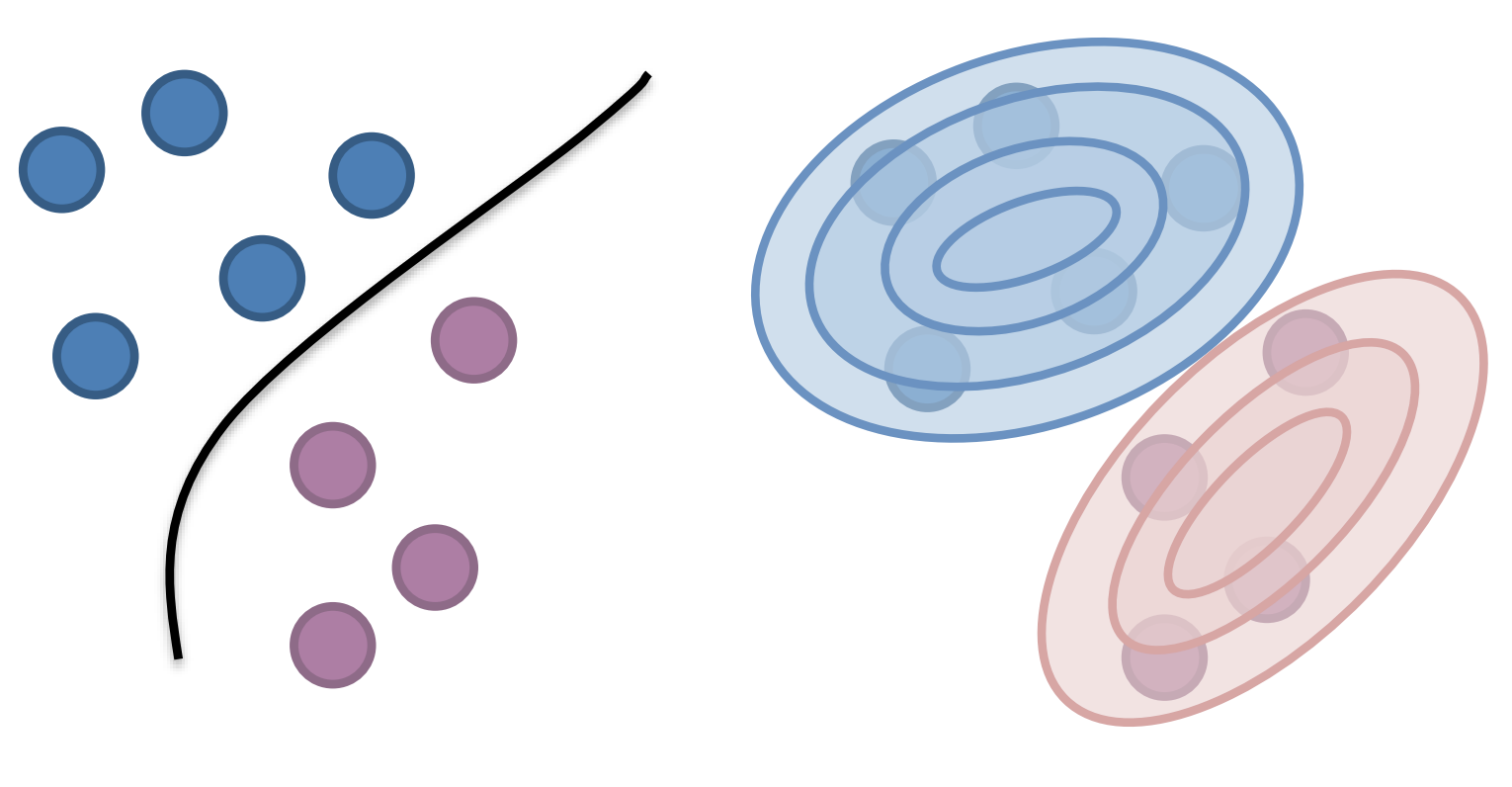
Fig. 8.1 A discriminative model (left) and generative model (right)#