19. Recommender Systems

As the final main module of our book, we want to explore the ever-present concept of recommender systems. Recommender systems are quite a broad set of applications of machine learning, and there are no shortage of examples you are likely familiar with in your experience online. These include, but are no way limited to:

• Netflix recommends movies/shows that it think you will watch.

• Spotify recommends artist or songs similar to ones you’ve listened to before. They even build playlists such as “Discover Weekly” to accumulate many of of these recommendations in a single playlist.

• Youtube recommends videos on your home page for you to watch, as well as set of videos for you to watch next related to the content you are currently watching.

• Social media companies like TikTok, Twitter, Facebook are constantly recommending you posts or media that they think you will like. Additionally, they recommend ads personalized to you based on the content you frequently interact with.

• Online stores such as Amazon recommend products they think you will purchase.

• Search engines serve you tailored ads based on your current search, and your search history.

As you can see, this concept of “recommendation” is quite broad topic and can be used in quite a few applications. However, a lot of these problems can be framed as special cases of the same underlying recommendation problem.

We will explore a wide set of possible algorithms for this recommendation framework in this chapter, and importantly, discuss the pros and cons of the various approaches based on their designs. For each of the approaches we outline, we will include a couple tags for the approach that we will define in detail later in the chapter, so you can ignore those for now on your first read.

19.1. Recommendation Framework

Fig. 19.1 Netflix rating buttons

Most recommendation problems can be framed in a similar framework of a user-item interaction matrix. We usually consider a system with \(n\) users and \(m\) items. In many settings we assume there are far more users than items (\(n \gg m\)). For example, in 2023, Youtube had approximately 2.6 billion user and 800 million videos (source).

Based on pairs of user/item interactions, our goal is to find some sort of measure of user preferences to make predictions about what to recommend. For example, suppose we were interested in seeing how Netflix users can rate items (movies) on a scale from “Not for me”, “I like this”, “Love this!”, which we will arbitrarily assign the values -1, 1, 2. We will use the value 0 to indicate a user hasn’t rated a movie.

Table 19.1 Example Netflix ratings user-item interaction matrix

	Item 1	Item 2	…	Item \(m\)
User 1	2	0	…	1
User 2	0	-1	…	0
…	…	…	…	…
User \(n\)	1	1	…	0

An important note is that what you choose to record and define interactions with users and items will have a tremendous impact on the model we learn and recommendations we make. Importantly, we should distinguish between two types of interactions we could record: implicit user feedback and explicit user feedback. Explicit feedback is when the user explicitly tells us if they like an item or not (e.g., Netflix users rating a movie as one they enjoyed or not) while implicit feedback are values we derive from their interaction with an item (e.g., did they go on to continue to use the service and watch more movies later). In different settings, we might care about different metrics for defining user interactions, and we will see the ramifications of the metrics we choose to measure.

Here are some example types of feedback that you could imagine gathering in various contexts. Note that there are multiple options for each application as we might care to optimize for different types of user feedback depending on context.

Table 19.2 Example metrics for measuring user-item interactions

Application	Users	Items	Metric	Type
Netflix	Subscribers	Movies/Shows	Rating	Explicit
			Watch time	Implicit
TikTok	Users	Videos	Hearted video	Explicit
			Followed creator	Explicit
			Watch time	Implicit
Amazon	Customers	Products	Purchased	Explicit
			Clicking on product	Implicit

It’s important to highlight the role that the metric we choose to optimize recommendations for, and the effects that has on our system. Most real-world systems might combine many of these metrics in a complex way. Specifically in cases of implicit feedback, these metrics are often proxies that might not align with the users’ actual preferences. For example, a recommendation system in Youtube to maximize watch time might not recommend content the user enjoys or will benefit from, but the most addicting content to get them to stay on the system longer. We will discuss the impacts the choice in metric we care to measure later on in the chapter.

The general learning task for recommender systems is: Given a user \(u\), recommend \(k\) items \(\{v_1, v_2, ... v_k\}\) that the user will prefer the most (according to our metric recorded in interaction data). Some recommender systems use outside information about the user (e.g., information provided in their profile or inferred from other sources), while others work directly with this user-item interaction exclusively. A special case is with \(k=1\), where recommend a single item, but many systems use some small \(k\) to recommend a set of items.

General Discussion

We will note that all of the specific algorithms we will mention in this chapter are fairly generally, but probably not used exactly as described in practice for real systems. The reason being, more often than not, a good recommendation algorithm is the secret-sauce for making a company’s product successful. For example, TikTok is commonly cited as booming in the social media space because of its incredibly sophisticated recommendation algorithm to recommend videos without much explicit feedback. Naturally, many companies use a lot of tricks and techniques they do not share with the public to keep that secret-sauce, well, secret.

However, that doesn’t mean there isn’t anything to discuss! There are a lot of common themes for design choices across various recommendation systems, and our goal is to try to give an overview of “canonical” methods and discuss their tradeoffs. Yes, most deployed models will be different in a myriad of ways from the foundational algorithms we describe, but understanding the choices and tradeoffs between different styles of recommender systems is useful in determining the choices you will want to make in your own systems.

In most contexts, this user-item interactions matrix we record in our system is incredibly sparse: users interact with a tiny minority of the total content on the system. This poses a challenge in that for each user, we have a tiny fraction of possible interactions to work from.

19.2. Approach 1: Popularity Recommendations

Tags

• Collaborative Filtering

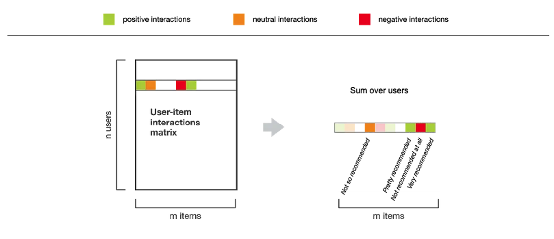
Perhaps the simplest approach to a recommender system that handles this sparsity problem is the popularity model. When we want to recommend an item (or set of items) for a user, we simply recommend what is globally popular in the system. That is, we completely ignore the concept of a input of a user \(u\), and recommend everyone the items that are globally most popular.

We can accomplish this by taking our user-item interaction matrix and summing across the rows to get a “total interaction” across all users. A sum is appropriate here instead of an average since we are intentionally trying to hype-up items that are popular across all users, rather than items that have a high average interaction from a single user really liking that one item. Usually we have added logic to avoid recommending an item that the user has already interacted with, but that is an optional implementation detail.

Fig. 19.2 Popularity Model (edited from source)

Let’s consider the pros and cons of a model such as this one for a recommender system. We will go through this exercise for all of the models we introduce to get a sense of their benefits and limitations. Each of these sections will ask you to pause and think about the pros and cons before reading our descriptions. Expand the boxes after taking some time to think of some benefits and downsides before moving on.

Pros

• Incredibly simple to describe and implement.

• While partially a con as we will describe in the next dropdown, the fact that the popularity model doesn’t personalize to each user can sometimes be seen as a benefit in a couple of scenarios. Two that come to mind are:

  1. When you first launch your application, you might not have enough data to make a more nuanced recommender system so it can be a decent starter-system to gather data initially before you can build something more complex.

  2. Many of our recommender systems will suffer from what is called the cold-start problem, where it’s not clear what to recommend when a new user or item enters the system. Since there is no personalization to the user, we naturally avoid the cold-start problem of not knowing what to recommend a newly-joined user.

Cons

• Clearly, the popularity model doesn’t take into account a particular user’s preferences at all. This extremely limits the recommender system since it cannot recommend anything more personal for a user.

• A popularity model is very susceptible to feedback loops, where its recommendations form a self-fulfilling prophecy that further reinforces the popularity of the items it recommends. If it only recommends popular content, then people will continue to watch that content, further increasing its popularity and making it more likely to be recommended in the future.

• Top-k recommendations can potentially be very redundant. For example, when a new Hunger Games movie comes out, the other movies tend to surge in popularity. In some cases, for extremely popular series, this can lead to a lack of diversity of items in the recommendations since, as we mentioned, popular content tends to get more popular in these popularity model systems.

The point we made above about feedback loops is important enough to highlight in the main text. In every recommender system we will discuss, the concept of a feedback loop will be present and important to consider. Broadly, a feedback loop results when the recommendations or outputs of the model will affect the future inputs of that model, potentially leading to cascading unintentional consequences. Earlier, we saw the non-recommendation system context of feedback loops in predictive policing and how predictions of increase crime lead to more police being deployed there, thus catching more (nuisance) crimes and justifying even more policing in those neighborhoods. Feedback loops are almost always unintentional consequences of the model using its outputs as inputs. But these cases are essentially unavoidable in most real world systems. Consider how almost the entirety of TikTok’s success relies on the recommendations it makes driving the vast majority of user interactions. While feedback loops are essentially unavoidable, that doesn’t mean we shouldn’t try to build safeguards in our systems to mitigate their impacts.

19.3. Approach 2: Nearest Users

Tags

• Collaborative Filtering: User-User

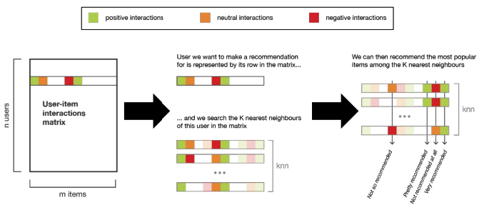
To add personalization to our recommender system, we consider an alternative model that uses our trusty k-nearest neighbor (kNN) algorithm to make recommendations for a user based on similar users. Given a user \(u_i\), compute their \(K\) nearest neighbors (note capital \(K\)) in the system, and recommend the \(k\) items (note lower \(k\)) that have the highest interactions amongst those \(K\) users.

Fig. 19.3 Nearest Users (source)

Let’s consider the pros and cons of a model such as this one for a recommender system. Expand the boxes after taking some time to think of some benefits and downsides before moving on.

Pros

• Pretty easy to describe and implement

• Adds personalization! You will get tailored recommendations based on users like you!

Cons

• Nearest neighbors might be a bit too similar, and limit the ability to make diverse recommendations. For example, if you and your nearest neighbors have interacted with only the same subset of content, then we can’t really make any meaningful recommendations. This technique relies on your nearest neighbors being similar, but not exactly the same as you. This is possible to fall apart in settings when there are far fewer users than content (potentially only interacting with content previously recommended to you as well).

• This technique also creates its own feedback loop. In particular, it can lead to echo chambers where users are siloed off to their own subsets of content. This is increasingly a challenge in many online systems that have resulted in the radicalization of certain subgroups due to only being exposed by their interaction with that radicalizing content (think reinforcing behaviors of conspiracy theory groups).

• These systems have the same scalability challenges that k-NN has in general. Prediction time is slower (unless using approximate methods) since you have to search over the whole dataset every time you want to make a prediction.

  • Also suffers from the curse of dimensionality since every user is represented in item-space (\(u_i \in \mathbb{R}^m\) where \(m\) is the number of items).

• The cold-start problem affects this model when new users are added to the system. If you just joined, who should we define your nearest neighbors to be if we have no data to base your similarity to other users on. This will be a common challenge with most of our recommender systems.

19.4. Approach 3: “People who bought this also bought…”

Tags

• Collaborative Filtering: Item-Item

A slightly different approach is to focus on the similarity of items rather than the similarity of users. A potential item-item recommender system is designed to fill in the blank of the sentence “Users who bought this, also bought…”

Fig. 19.4 Amazon’s Item-Item recommendations of “Frequently bought together”

One way of implementing this model is to consider the co-occurrence matrix \(C \in \mathbb{R}^{m \times m}\) where \(m\) is the number of items in the system. Each entry \(C_{i,j}\) counts the number of users who bought both item \(i\) and item \(j\). Note that \(C_{i,i}\) is the total number of users who bought item \(i\). For the recommendation task, we are given an item \(i\) and can predict the top-\(k\) items that are bought together with item \(i\) (usually excluding \(i\) as an option).

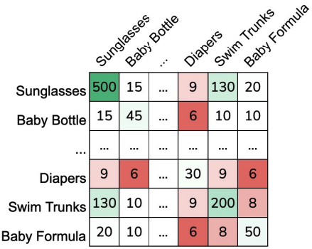
Fig. 19.5 A co-occurrence matrix for items (\(C \in \mathbb{R}^{m \times m}\))

One difficulty that arises with a co-occurrence matrix like t his is that globally popular items will drown out items since their counts are naturally larger. One solution that ignores the global popularity of items and makes item recommendations more specific to the input item is to scale all of the counts. One common scaling is the Jaccard Similarity we described earlier. The scaled co-occurrence matrix \(S\) can be found with

\[S_{i, j} = \frac{\text{# purchased}\ i\ \textbf{and}\ j}{\text{# purchased}\ i\ \textbf{or}\ j} = \frac{C_{i, j}}{C_{i,i} + C_{j,j} - C_{i, j}}\]

Below we show the same co-occurrence matrix data but scaled with the Jaccard Similarity.

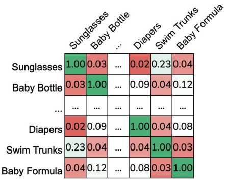
Fig. 19.6 A co-occurrence matrix for items scaled with Jaccard Similarity (\(S \in \mathbb{R}^{m \times m}\))

It is also possible to augment this procedure to explicitly add user personalization by incorporating their interaction history in the average. Instead of reporting the items that have the highest co-occurrence, we can compute a score for each user and an item based on their history. For example, if we know a user has only bought a baby bottle and baby formula, we could incorporate that to only use those in the computation for a score for each item. In this example, we could define the score for a user and the item “diapers” as follows (assuming they have only bought a baby bottle and baby formula).

\[Score(u, v=\text{diapers}) = \frac{S_{diapers, baby bottle}}{2} + \frac{S_{diapers, baby formula}}{2}\]

Our recommendation algorithm could then return the \(k\) items with the highest average score. As an additional implementation detail, you could also do a weighted average to put more weights on recent purchases.

Let’s consider the pros and cons of these approaches.

Pros

• Provides personalization based on the item the user is looking at. Can also add personalization to the user by incorporating and adding more weight on the user’s previous interactions.

• Slightly more scalable than Nearest User in many real-world settings since we often assume the \(n \gg m\). Representing a \(\mathbb{m \times m}\) matrix is generally more efficient than our \(\mathbb{R}^{n \times m}\) matrix for Nearest User.

Cons

• Still suffers from feedback loops, in that it generally recommends items that are globally popular since they are more frequently bought with other items.

• Still has some scalability issues. While better than Nearest User in terms of memory requirements, storing the whole item-item matrix is quite expensive in real-world settings.

• Suffers from the cold-start problem, but when new items are added to the system.

19.5. Approach 4: Feature-Based Approaches

Tags

• Feature-Based or Content-Based

Also referred to as content-based approaches

One common limitations of the models we discussed earlier is they rely solely on information from the user-item interaction matrix and do not use any extra information in their predictions. What if we tried to also include standard machine learning approaches we have discussed in this book to make a model to make predictions based on features we derive about the user and/or items?

1. Recall you would need to handle categorical features with something like a one-hot encoding.

For example, we can create a feature vector \(h(v)\) for each item in the catalogue that describes various attributes of each item^{1. For simplicity, let’s ignore personalization to a user and form a global model of interactions with an item based on its features.}

Table 19.3 Example features for a Movie catalogue

Genre	Year	Director	…
Action	1994	Quentin Tarantino	…
Sci-Fi	1977	George Lucas	…
Drama	2017	Greta Gerwig	…

Assuming our feature vector is \(d\)-dimensional (\(h(v) \in \mathbb{R}^d\)), then we can learn some sort of global model to make predictions about interactions with that item. For simplicity, let’s assume we are using a linear model, but more complex models could also be used. In that case we now need to learn coefficients for our model

\[w_G \in \mathbb{R^d}\]

Which can do with a modified version of our OLS problem that minimizes squared error across the (user, item) pairs we have interaction data for. We use the notation \(u, v\) to be a pair of user/item, \(r_{u,v}\) to indicate the interaction metric for that user and that item, and \(r{u,v} = ?\) if the user has not interacted with that item. We can additionally add regularization to our model to instead of using plain OLS, using some sort of regularized regression of our choosing.

\[\hat{w}_G = \argmin{w_G} \frac{1}{\text{# ratings}} \sum_{u, v:\ r_{u,v} \neq ?} \left( w_G^T h(v) - r_{u, v}\right)^2 + \lambda \norm{w_G}\]

Note that a major limitation of this global model is it can’t take into account user-specific preferences for certain items. However, we can modify this model to account for that in a couple of ways.

The first way is to include user-specific features in our data and learn coefficients for those as well. So for example, we might have the following dataset of item features and user features.

Table 19.4 Example features for a Movie catalogue with User features and Item features

Genre	Year	Director	…	Gender	Age	…
Action	1994	Quentin Tarantino	…	F	25	…
Sci-Fi	1977	George Lucas	…	M	42	…
Drama	2017	Greta Gerwig	…	M	22	…

We would represent this new set of features as a combination of both user features and item features \(h(u, v)\). Our global model would now be the following, noting that we change all of our dimensions for \(w_G \in \mathbb{R}^{d_1 + d_2}\) where \(d_1\) is the number of user features and \(d_2\) the number of item features.

\[\hat{r}_{u, v} = \hat{w}_G^Th(u, v)\]

While this approach is the simplest way to include user features, it tends to not be used in practice because it suffers from the cold start problem. What feature values for the user-features do we use for a brand-new user that signs up for the service if we don’t have that information yet?

We can actually avoid this user cold-start problem by changing our learning task just slightly. Instead of including user-specific features into our global model, we will restrict our model to only using item-specific features. But to learn personalization for the user, we will mix in a user-specific model the predictions for the global model. One such example is called a Linear Mixed Model or Linear Mixed Effects that combines the results of two different models in a linear fashion. We will learn our global model \(\hat{w}_G\) that takes item features \(h(v)\) to make predictions. On top of this, we will also learn a user-specific model \(\hat{w}_u\) that works of the same set of features, but makes predictions tailored to that user \(u\). Then, our overall prediction for \(\hat{r}_{u, v}\) is as follows.

\[\hat{r}_{u,v} = \left( \hat{w}_G + \hat{w}_u\right)^T h(v)\]

You can think of this as modifying the global model to have coefficients that are more tailored to the individual user \(u\). When a new user joins, we can simply set \(\hat{w}_u = 0\) and provide no personalization to start. As the user interacts with more and more items, we can continuously update their coefficients to provide more tailored results. Some practical details for how we can train this user-specific model \(\hat{w}_u\):

• We don’t have to retrain the user-model from scratch, but instead can train it on the mistakes or residuals of the global model. This is a slight simplification of the task to essentially finding the deviation of the user from the global “average” user rather than learning their coefficients from scratch every time.

• We can do more complicated Bayesian-style updates that start of deviations from the global model to be small, and allow them to get larger and larger as we are more confident in a user’s history.

Again, let us consider the pros/cons of this feature-based approach.

Pros

• No cold start problem! As described, the user-deviation approach allows us to make global recommendations for new users. We will note that this discussion has assumed the item-features are provided, but this is a common assumption in that items are often approved in the app or uploaded with a set of known features. For example, in TikTok creators uploading videos tag the video for TikTok about the contents and topics of the video.

• It provides personalization based on the user’s characteristics and the item’s characteristics.

• Extremely scalable since we only need to store the global model weights and user-specific model weights.

• You can add as arbitrarily complicated features as you want to your model. For example, you might know that user preferences change throughout the day or based on the time of year. You can include those as features in your model to hopefully learn more complex macro-trends in preferences.

Cons

• By far the biggest downside of this model is it requires a lot of manual work. Defining which features to include and why is challenging, and in many settings getting quality data for each user and item is quite difficult. So unless you have high quality data sources that can predict user preferences well, these approaches might just be less accurate than more simple approaches we discussed earlier.

19.6. Approach 5: Matrix Factorization

Tags

• Collaborative Filtering: Model Based

Coming soon